Constraining Nanoflare Heating Frequency with a Global Active Region Model
Will Barnes, Stephen Bradshaw
Rice University, Houston, TX USA
8th Coronal Loops Workshop – Palermo, Italy
28 June 2017
Heating Frequency in AR Cores
- What is the frequency of nanoflares in AR cores?
- Define heating frequency in terms of
– high-frequency heating– low-frequency heating
- Emission measure slope
,often used as a diagnostic for heating frequency - Many factors hinder interpretation
- Multiple emitting structures along the LOS
- Nonequilibrium ionization
- Inversion techniques for finding EM
- Lack of spectral coverage in detectors
Two primary questions:
What are the observational signatures of nanoflares of varying frequency?
Are these signatures detectable?
Forward Modeling Global Active Regions
synthesizAR– a Pure-python pipeline for producing forward-modeled instrument data products from field-aligned loop hydrodynamics- Relies heavily on the widely-used and well-documented scientific Python stack
- Workflow
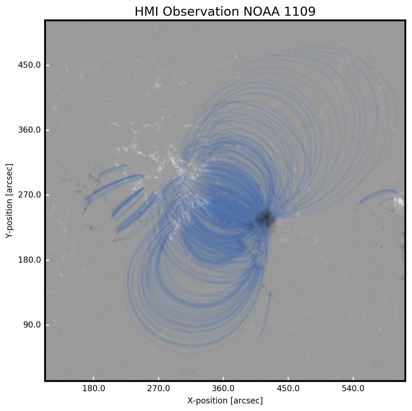
- Select HMI observation of an AR and perform field extrapolation
- Configure loop simulations from field extrapolation results
- Load simulation ouput and map to fieldlines
- Synthesize emission for each spatial point and timestep
- Project along LOS and output data product (e.g. FITS)
- Build up a global active region model from an ensemble of hydrodynamic loop models
Model Setup
- Use AR NOAA 1109 (#9 in Table 1 Warren et al., 2012) from 29 September 2010
- Model 103 independently evolving fieldlines with two-fluid EBTEL model for ≈2×10⁴ s
- Calculate emission from all ions in the CHIANTI database (AIA)
- Synthesize wavelength-resolved intensity for 22 transitions (EIS)
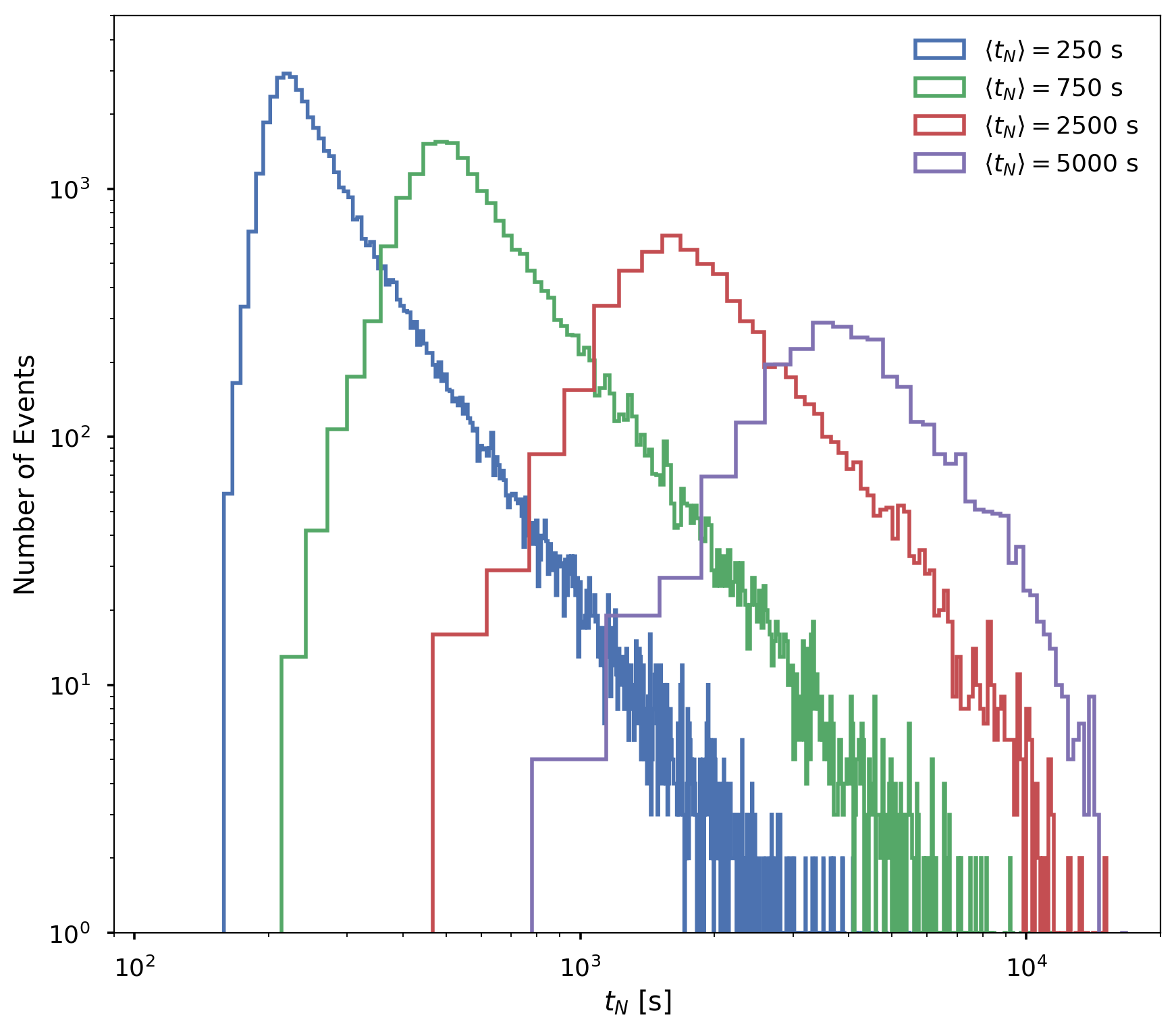
- Repeat for four different average waiting times,
Hydrodynamic Loop Model
Two-fluid EBTEL model of Barnes et al. (2016a),
Heat electrons or ions dynamically and model spatially-averaged coronal quantities
Spectroscopic Details
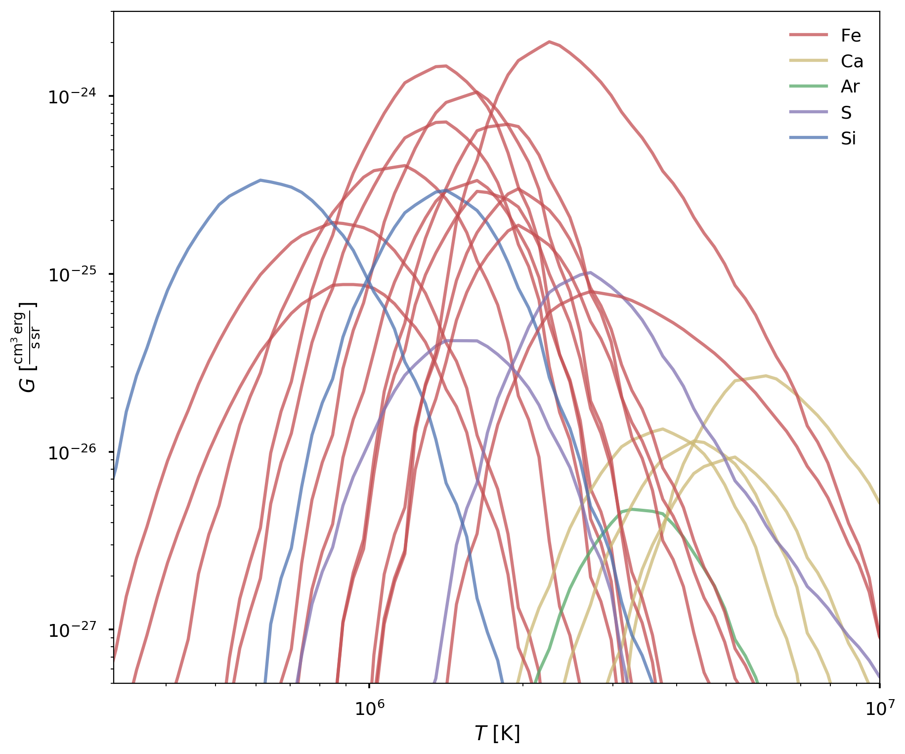
| Ion | Wavelength | Ion | Wavelength |
|---|---|---|---|
| S X | 264.2306 | Si X | 258.374 |
| Fe X | 184.537 | Fe XII | 195.119 |
| Fe IX | 188.493 | Fe IX | 197.854 |
| Fe XII | 192.394 | Fe XVI | 262.976 |
| Fe XI | 180.401 | S XIII | 256.6852 |
| Ca XV | 200.9719 | Fe XV | 284.163 |
| Fe XIII | 202.044 | Fe XIV | 264.7889 |
| Fe XIII | 203.826 | Ca XVI | 208.585 |
| Fe XIV | 270.5208 | Fe XI | 188.216 |
| Ca XVII | 192.8532 | Si VII | 275.3612 |
| Ca XIV | 193.8661 | Ar XIV | 194.401 |
Heating Parameter Space
- Each strand heated independently
- Preferentially heat electrons
- Triangual pulses with duration
- Total input energy per strand set by
- Event energies chosen from a power-law distribution with
such that larger events require a longer "winding time"
Emission Measure Diagnostics
- True emission measure from simulated thermodynamic quantities,
- Bin in temperature
with width - Predicted EM from regularized inversion code of Hannah and Kontar (2012)
- Assume 25% uncertainty on our intensities to balance acceptable
and smoothness - Apply to pixel-averaged and full AR
- Assume 25% uncertainty on our intensities to balance acceptable
- Fit power-law to cool side such that
- Fit between 1 MK and
(4 MK true, 3 MK predicted), where - Only fit to pixels where
cm-5 and acceptable fit
- Fit between 1 MK and
Pixel-averaged Emission Measures
- Warren et al. (2012) constructed
from pixel-averaged intensities in NOAA 1109 using MCMC - Time-average integrated intensities (over 5000 s interval) for same set of spectral lines
- Compare predicted and true EM with predicted EM derived from reported intensities
Global AR Emission Measure – True
Global AR Emission Measure – Predicted
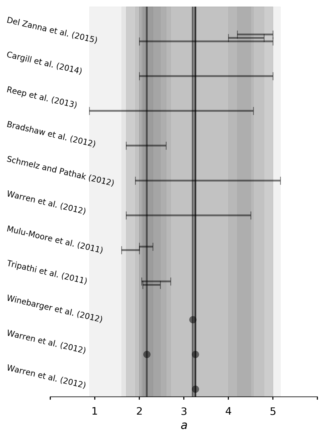
Emission Measure Slopes
Emission Measure Slopes
Conclusions
- Global active region modeling a powerful tool for studying dynamically-heated AR cores
- Efficient
- AR Geometry
- Detailed loop physics (with 1D models)
- Atomic physics and instrument effects
- Relationship between predicted
andmuch "messier" compared to true - Predicted EM peak at lower temperatures than true EM, independent of heating frequency
- Observed slopes most consistent with intermediate to low frequency heating, but spread is large
- Caution when computing emission measure from model results